

Although the world appears a very turbulent place, financial volatility is currently rather low. How do we know this? One method widely used by commentators and market analysts is to refer to a measure of global risk aversion called the VIX. This post explains how can we infer something about market participants’ attitudes to risk, based on option pricing theory and the existence of heavily traded option markets. It won’t try to answer the more profound question, why is volatility so low?
What does risk aversion mean?
A central assumption in financial economics is that people don’t like risk. That might seem obvious, but it’s worth fleshing out the idea a bit more. Risk sounds like a bad thing and there are good evolutionary reasons why humans don’t like risk, such as prefering to know for sure whether a patch of long grass contains a predator or not. The human who took the view that there was a risk and so avoided the grass will on average live to tell the tale, even if he or she is wrong much of the time, and pass on their genes. The curious human who didn’t mind the risk eventually got eaten and so their genes didn’t survive.
The economic theory of decision making under risk measures it as the variation in outcomes. So in the world of finance we can measure the average return on say equity shares and we can measure the variation of those returns, defined as the standard deviation, which is a mainstream statistical measure of how far a variable deviates from the average over a period of time. If we assume, plausibly, that investors like higher average returns but don’t like a higher standard deviation of those returns, then we have the basis of a theory.
The exact definition of risk aversion is a bit more complex and it turns out that there are many complications to the simple statement that investors don’t like risk. For example, do investors have varying levels of risk aversion in relation to their income or wealth? We might reasonably think that a poor person is much more risk averse than a rich one, since a rich person can afford to take some risk without losing too much of their wealth. A poor person by contrast only needs a single piece of bad luck to suffer destitution or even death.
To make the concept a bit more precise, economists think of risk aversion as the willingness of a person to give up an amount of return to avoid an amount of risk. Equivalently, a risk averse person would prefer a certain outcome, say a return of 5%, to a higher average expected return, say 6%, that comes with a possibility of doing worse than 5%. The idea is familiar from TV game shows where a contestant who has reached a certain stage of the game is offered a prize if they quit at that point. But if they continue they might win a much bigger prize; however, they might also go home with nothing. A risk averse person would take the lower but certain prize rather than go for the further stage of the game in which the expected payoff might be much higher. These games are complicated by the possibility that skill is involved: if the contestant is confident of doing well then taking the further stage is not so risky. And in a TV game contestants are to some extent encouraged to take risks that they might not take in everyday life.
The quantity of risk aversion is how much expected return a person would give up relative to a certain return. There is no particularly rational point of risk aversion, it depends on a person’s situation and on their psychology, which might reflect their history and genetics (there is evidence of a biological aspect to risk aversion, meaning we may be born with a particular level). A person might be confronted with a safe and certain return of 2% in a government-insured bank account, compared with 7% average expected return on investing in the stockmarket. So the risk premium is five percentage points. Is this enough to compensate the investor for taking the risk that occasionally the stockmarket falls 5% and very rarely 10% or even 20%? We can’t answer this definitively. We can only observe that most investors, when they are truly investing as opposed to gambling (when the element of risk is exciting and actually makes the trade more interesting and enjoyable) would need at least some extra expected return as compensation for taking the risk that the return could be lower than the return on the safe bank account.
How option prices help to reveal risk aversion
Ordinary share prices move up and down all the time but tell us little about the risk attitudes of investors. The value of a share in theory reflects the flow of expected future dividends, discounted by an appropriate rate of interest which captures the riskiness of that dividend stream. A change in share prices can be caused by a change in expectations about future dividends (e.g. because a company announces better than expected profits) OR by a change in attitudes to risk, which alter the discount rate, OR by both at once. It’s hard to disentangle these two forces.
Options are securities which grant the owner the right, but not the obligation, to buy or sell something, such as a share. So a call option on XYZ shares at a strikeprice of 106p mean the owner can buy XYZ shares in the market at 106p, whatever the current share price. If that price is above 106p then the option is clearly worth something. But it is also worth something even if the current share price is below 106p, so long as the option has some time to run before expiry. Why? Because during the period the option exists, there is a possibility that the shares will rise above the strike price and then the option will have value. How likely is it that the shares move up above the strikeprice? It’s more likely to happen if the shares are volatile, meaning they swing around up and down. Nothing is guaranteed, but you’d probably pay more for an option on a volatile share than a very stable one, all else being equal, because there is a greater chance that the volatile share will rise above the strikeprice. Even if that’s only temporary and the shares then fall in value, you have a moment when you can exercise the option and make a profit. The chance of that profit being available is the value of the option.
It’s the same idea as the value of insurance. You would value fire insurance more (and be willing to pay more for it) if you though the likelihood of a fire was greater. Fire insurance is a form of put option, meaning that you can in effect sell your house to the insurance company at its replacement value, if it’s damaged by fire. If you think a fire is very unlikely you may not think it’s worth taking out fire insurance, which is in fact pretty rare. But most people pay for it because the cost if it does happen is so disastrous for an average household – a reflection of risk aversion.
All else being equal, investors are more likely to buy options, which can be used as protection against risk, the more they fear that risk. Periods of stock market turbulence of fear of future turbulence make options more valuable. So there is a broad link betwen the price of options and investor attitudes to risk.
Volatility makes options more valuable
The original theory of option pricing, known as Black-Scholes-Merton (BSM) after its founders, has a number of variables, including the volatility of the financial asset on which the option is created (“written”). So we can say that the value of an option on XYZ shares is a function of several things, including the volatility of XYZ shares. We measure the volatility as the standard deviation of the shares during a period of time, perhaps the five years of trading history up to the present. That’s our best guess of the volatility of the shares in future, which is of course what we really care about. A higher volatility, all else being equal, raises the value of the option. Why? Consider our XYZ case again. The current share price is 100p but the strike price of the call option is 106p. How likely is it that the share price will go above 106p, in which case the option is in-the-money, meaning you can sell it immediately for a guaranteed profit?
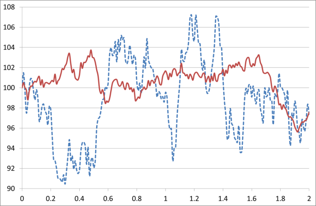
That’s more likely to happen if the shares are more volatile. If they are very stable then over say a year they’re unlikely to move much above 100p. But if they’re highly volatile then it’s more likely that they will occasionally (and perhaps briefly) move above 106p (and at times of course fall well below 100p). The chart below illustrates two versions of XYZ shares. The red, continuous line is a low volatility path for the shares starting at 100p, for 200 time periods. The blue, dotted line shows a higher volatility case. Over a period of 200 time periods (which could be hours or days) the shareprice moves up and down randomly but with a fixed volatility. The more volatile share naturally moves up and down a lot more than the less volatile but during this period it is sometimes above the strike price and could then be exercised for a profit. The less volatile share never reaches the exercise price and never makes it into profit.
Note that both of these share paths are simulations in Excel, using the simplest model, the geometric Brownian motion(*). That model assumes that a share moves each period randomly up or down with a fixed standard deviation. Usually a share also has a trend movement (known as “drift”) but I’ve set that to zero in this case to emphasise the pure randomness. This model is somewhat simple, since there is evidence that volatility is not constant. It can vary over time or can even be itself random. Models with these features provide a better fit to actual shareprices but they are mathematically more complicated.
These shareprice paths are illustrative. Anyone buying the option doesn’t know what will happen to the shareprice. But they do know that the more volatile shareprice path has a greater probability of reaching the option strike price and that makes them willing to pay more for that option than for a less volatile shareprice path. It is a pure coincidence that by the end of the 200 periods both share paths show a fall to about 98 pence. There is an infinite number of possible shareprice paths that we can generate using this sort of simulation, I’ve picked a couple that illustrate my point but it could be that in some cases the low volatility path reaches the strike price and the high volatility path doesn’t, such is the nature of randomness. But on average we can expect the high volatility path to reach the strike price more often than the low volatility path, which is what should guide a rational investor.
Implied volatility: the volatility the market expects that justifies current option prices
If options are traded in financial markets, we can observe the value that the market puts on a particular option such as XYZ. If we’re confident that our option pricing theory is correct, we can then invert the calculation and ask the question, what level of volatility is required to make the option value observed in the market fit the theoretical value? We know the other ingredients in the option valuation model such as the interest rate, the current stock price and the exercise price. The only thing not directly observable is the future volatility of the share expected by the option traders. But that is what we can infer from the market value of the option.
There are options traded on most of the world’s largest quoted companies. And there are options on groups of companies, including on broad indices of stocks. So just as you can invest in the S&P 500 index as a way of buying exposure to the largest stocks in the US stockmarket, you can buy an option on that index,meaning that you would have the right to buy the index at a predetermined strike price. Why might you do this? Well you may have already decided that you want to put some money into the US stockmarket but it takes time to sell other investments to realise the funds to do so. For a smaller amount of money you can buy an option to purchase the S&P500 index at a price just above the current level, so that if the index starts rising and running away from the level at which you’d intended to invest but don’t yet have the funds to do so, you’ve bought yourself protection, meaning you’ve insured yourself against the rising index. If the index falls or stays level then your option may expire worthless but the cost of the option is in effect an insurance premium that is the price of sleeping soundly until your money becomes available.
The VIX: a measure of market expectations of volatility
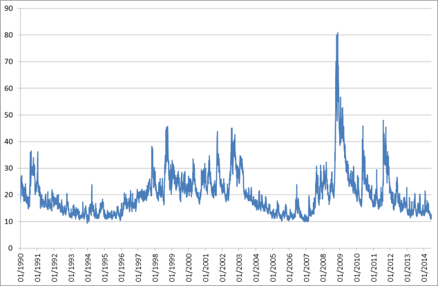
At any moment in time there are various different options on the S&P500 being traded. The Chicago Board Options Exchange (CBOE) takes these options and calculates from each of them the future volatility of the S&P500 index which the option price implies, using a version of the BSM option pricing model. This is known as implied volatility: the volatility of the S&P500 index that the market prices of options imply investors are assuming about the future. That implied volatility is then distilled into the VIX index, which has been published since 1990. Changes in the VIX tell us about the changing volatility views of investors as a group. Broadly speaking, higher implied volatility corresponds to higher levels of investor fear or anxiety. So a higher value of the VIX means investors collectively are more anxious about the future. The VIX is based on options with 30 days to expiry so it’s a way of inferring market expectations of stock market volatility a month ahead. This can be interpreted, broadly as a measure of global investors’ average level of risk aversion.
So if the VIX is a measure of market fear, what is it telling us? The chart below shows that we are back to the levels of 2007, before the great spike during the global financial crisis. Does that mean everything is OK with the world of finance? Unfortunately not, but that’s another story.
Additional reading
The Federal Reserve Bank of New York’s Liberty Street blog reports a research study that attempts to match large changes in implied volatility (where “large” means two standard deviations away from the previous 60 day average) to key surprises such as a change in Fed monetary policy, arguing that such shocks make investors temporarily more risk averse and the increase in implied volatility is a reflection of that.
(*) Using Excel’s RAND function to generate random numbers and NORMSINV to turn these into a Gaussian normal distribution. The process is dSt = μStdt + σStdWt, where Wt is a Wiener process. The drift μ is set to zero and volatility σ is set to 0.05 in the low volatility case and 0.15 in the high volatility case.